Day 7: A Top Trending Python Package

Note: We apologise we’re delayed by a few days. Our Chief Writer John has been unwell this week. Like any confectionary advent calendar, you can enjoy bingeing on multiple morsels per day this week as we catch up.

Today’s edition brings you a library that can be used equally for fun & profit. It provides access to a vast dataset of public interest and opinion, with applications ranging from politics and healthcare to tourism and finance.

Pytrends is an easy-to-use but unofficial library for interfacing with Google Trends including popularity of search terms over time, across different geographical regions (by country, region, city), and in various languages. It can also provide trending search terms, and related searches for a given term during a specific time window.

Here’s a few ideas of what you could use pytrends for:

1. 👥 Opinion polling & social science research: Analyse the public’s interest across many countries in a given set of topics over time.

2. 🔍  Market analysis: Identify emerging market trends or declining interest in product categories.

3. 🏥 Efficacy of public health campaigns: Track the popularity of search terms relating to health issues such as mental health or disease prevention to gauge public awareness and effectiveness of campaigns.

4. 🏖️  Travel & tourism industry analysis: Identify peak times of interest for various destinations.

5. 📝 Content strategy: Social media marketers, bloggers, and digital media companies can identify trending topics for content creation.

6. 👗 Fashion industry trend analysis: Brands and retailers can monitor the popularity of different styles of clothing, materials and patterns to inform decisions around future designs or inventory planning.

7. 🏡 Real estate market research: Track interest in specific locations or properties, understanding buyer profile and interests.

8. 💹 Financial market analysis: Investors and financial analysts can track interest in a given company or industry, by country or region, over time, to identify market sentiment and potential investment opportunities.

Step 1: Create a connection object

First, you will need a connection object. This could be as simple as

but you may want a few more bells & whistles to reduce the chance of being blocked by Google’s rate limit:

Here’s what each argument does:

• hl  –  host language for accessing Google Trends.

• tz  –  timezone offset, e.g. 0 for UK GMT or 360 for US CST.

• timeout – number of seconds your client will wait to establish a connection, and also how long it will wait to receive a response (see more in the requests docs).

• proxies  –  https proxies, must be https, and requires a port number.

• retries  –  Total number of retries for connecting to and reading from the remote source.

• backoff_factor

  • Most errors are resolved immediately by a second try. After this, a backoff factor is applied between attempts.

  • Calculation: backoff_factor * (2 ** (total_retries - 1)) seconds.

  • Example: backoff factor of 0.1 results in sleeping for [0.0, 0.2, 0.4, … ] seconds between retries.

• requests_args — dict with additional parameters to pass to underlying requests library such as verify=False to ignore any SSL errors.

Step 2: Prepare a payload

Next, prepare your payload. The example below requests a single keyword and a timeframe going back five years:

Here’s another example:

The .build_payload() method accepts the following parameters:

• kw_list  –  list of up to 5 keywords to search for, or topic identifiers supplied by using pytrends.suggestions()

• cat  –  filter results within a given category from this list

• geo  –  two-letter country abbreviation using ISO 3166-2 codes (including regional codes such as GB-SCT for Scotland)

• timeframe  –  defaults to last 5 years ( today 5-y ), other options include

  • all = everything

  • 2021-01-01 2022-12-31 = specific date range

  • 2023-12-10T10 2023-12-10T15 = specific UTC-based datetime range

  • today 3-m = last 3 months (1-m, 3-m, 12-m only)

  • now 7-d = last 7 days (1-d, 7-d only)

  • now 4-H = last 4 hours (1-H, 4-H only)

• gprop — Filter by Google properties such as images, news, youtube, froogle (defaults to web)

Step 3: Download Google Trends data

🗺️  What’s trending right now?

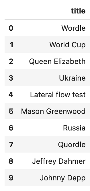
The .trending_searches() method highlights the top trending search terms right now, whilst the .top_charts() method indicates the top trending searches in any geography in a given year.

At the time of writing, the trending searches relate to Netflix thriller Leave the World Behind, Norwegian footballer Erling Haaland’s foot injury, and Japanese pitcher Shohei Ohtani joining the LA Dodgers. You can see the top charts for the UK in 2022 below (lots of Wordle and World Cup):

🗺️  Interest by region

Let’s compare popularity of the “Christmas” search term by country. The .interest_by_region() method returns a pandas DataFrame, so we can immediately query & sort the result. Note how the results are normalised with the top result being 100.

📈  Interest over time

In this example, we build a payload using two keywords (Python vs Rust). Two other things to note:

1. We’ve wrapped the pytrends code in a function in order to cache it. Given Google’s aggressive rate limiting, this makes sense especially when re-running code with the same inputs.

2. We’ve decorated the function using the joblib Memory class. If you read our previous issue, Cache Me If You Can, you might wonder why we haven’t used the built-in @cache decorator from functools. If you try this, you’ll see that @cache only works with hashable Python types, i.e. not the list expected by the keywords argument.

🌐 Related topics

If we look at the interest over time for elves we see an expected annual cycle of holiday-related searches every December. However, we saw multiple spikes in 2022…let’s investigate further using related topics.

Here we zero in on elves between 15th August to 15th September 2022, across all geographies, before requesting the top related topics during this period.

It looks like this acyclic September spike was caused by the release of The Lord of the Rings: The Rings of Power by Amazon Studios on 2nd September 2022. 🧝‍♂️👑🌋🔨🏞️🏰🛡️🧙‍♂️🌌✨🤝🔮👁️

👍  Are you enjoying our series?  ♥️

We love analysing trends, and we’d love even more to see the #PythonAdventCalendar trending by Christmas! If you’re enjoying the series,, then please share it on your socials, on your work Slack, and with your friends. You can find us @CoefficientData on Twitter and as Coefficient Systems on LinkedIn.

See you tomorrow! 🐍

Your Python Advent Calendar Team 😃